


ADAS dse
總需求和總供應是經濟學中一個重要的概念,是衡量一個國家或地區經濟活動的重要指標。
總需求是指一個國家或地區在一定時間內對財貨和服務的總需求量,而總供應則是指在同一時間內經濟體中提供的總貨物和服務的總數量。
總需求和總供應的變化對經濟體的穩定和發展具有重要影響,因此它們的分析和研究是經濟學研究的核心內容之一。
本文將介紹總需求和總供應的基本概念,並探討它們對經濟體的影響,以及相關的政策措施。
Aggregate demand
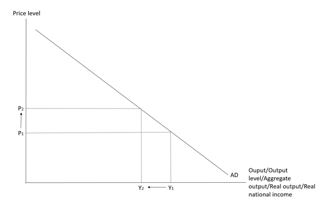
- It shows the relation between the price level and the aggregate output demanded in an economy, other factors being constant.
- Aggregate output demanded is the real output demanded by an economy at a particular price level over a specific period. It can be measured in terms of real GDP or real national income.
- Aggregate ouput demanded = C + I + G + NX
|
|
Movement along the AD Curve |
Shifting of the AD curve |
|
Cause |
Changes in price level |
Any non-price factors which would affect aggregate output demanded |
Reasons for the downward sloping aggregate demand curve
- Wealth effect:
As many assets in the economy are dominated in nominal values., the higher the price level, the lower the purchasing power of money. This reduces the wealth of the economy (in real terms). As a result, household and firms reduce their purchase of all goods and services and the real output drops.
- Interest rate effect:
As the price level rises, households and firms demand more money to finance their transactions. Given the fixed supply of money, the interest rate would rise. An increase in interest rate would cause decline in investment and consumption and also the real output.
- Net exports effect:
As the domestic price level rises, foreign-made goods become relatively cheaper so the quantity demanded of imports increases. However, the rise in domestic price level also means that domestic-made goods are relatively more expensive to foreign buyers so the quantity demanded of exports decreases. When the volumes of exports decreases and of import increases, net exports will decrease, so as the real output.
Non-price-level factors which would shift the AD curve
|
Factors affecting private consumption expenditure |
|
|
Disposable income |
Disposable income↓→C↓→AD↓ |
|
Desire to save |
Desire to save↑Proportion of disposable income↓→C↑→AD↓ |
|
Interest rates |
Interest rates↑→Cost of consumption↑→C↓→AD↓ |
|
Wealth |
Wealth→Ability to consume↓→C↓→AD↓ |
|
Factors affecting gross investment expenditure |
|
|
Interest rates |
Interest rates↑→Cost of investment↑→I↓→AD↓ |
|
Profit taxes |
Profit taxes↑→Less willing and able to invest →I↓→AD↓ |
|
Business prospects |
Less optimistic business →Less profitable to invest →I↓→AD↓ |
|
Factor affecting government consumption expenditure |
|
|
If the government raises government consumption expenditure, aggregate demand will increase, and vice versa. |
|
|
Factors affecting exports and imports |
|
|
Exchange value of trading partners |
Value of domestic currency relative to a foreign currency↑→Our imports become less expansive to our residents while our exports become more expansive to foreign residents →Volume of imports↑ and volume of exports↓→Net exports↓→AD↓ |
|
Price level of trading partners |
Foreign price level↓→Volume of imports↑and volume of exports↓→Net exports↓→AD↓ |
|
National income of trading partners |
National income of trading partners↓→ volume of exports↓→Net exports↓→AD↓ |
|
Trade policies |
Trade policies that can restrict our imports and promote our exports→Volume of imports↓and volume of exports↑→Net exports↑→AD↑ |
Aggregate supply
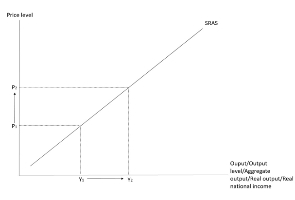
- It shows the relation between the price level and the aggregate output supplied in an economy, other factors being constant.
- Aggregate output supplied () is the real output supplied by an economy at a particular price level over a specific period. It can be measured in terms of real GDP or real national income.
|
|
Movement along the AS Curve |
Shifting of the AS curve |
|
Cause |
Changes in price level |
Any non-price factors which would affect |
Reasons for the upward sloping short run aggregate supply curve
- The imperfect adjustment of input prices
When the price level increases, the adjustment of input prices is imperfect/incomplete (e.g. due to the long term contracts of factors of production), so the real cost of production — i.e. nominal cost divided by the general price level – will fall. Firms would thus use more factor inputs to produce larger output. Therefore, the SRAS curve is upward-sloping, i.e. a higher price level would result in a higher output level.
- Sticky-cost (wage) effect:
The input prices are usually fixed during a short period under long term contracts. When P↑, output price rises more than input prices, so it is more profitable for firms to produce more, output level would thus rise..
Non-price-level factors which would shift the SRAS ONLY
These factors would not cause any change to the full employment output level/potential output level since the quantity of factor endowment, quality of factor endowment, production technology, production efficiency and infrastructures remain unchanged.
*Factor endowment refers to factors of production owned by an economy that can be used in production.
|
Factor costs |
Factor costs↑→SRAS↓ |
|
Supply shocks |
Negative supply shock →SRAS↓ |
|
Expectation of price level |
Expected price level↑→Firms retain more of their present supply for future sale→SRAS↓ |
|
Government policies with only short run effects on aggregate output supplied |
Production subsidies↑→Production costs↓→SRAS↑ |
Long run supply curve
- The LRAS curve is a vertical line and is positioned at the gull employment output level (YfS), meaning that all available resources are used efficiently.
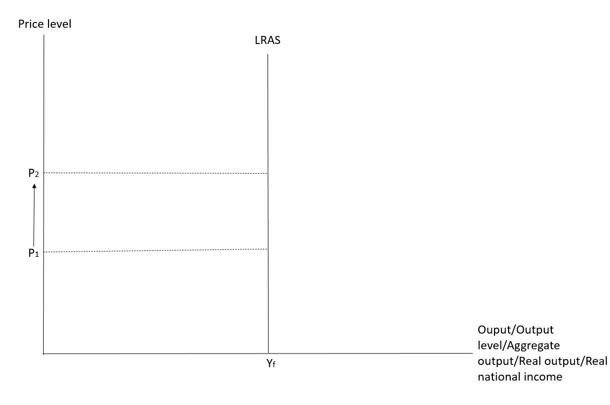
Reasons for a LRAS curve positioned at Yf
- Fully adjusted input and output prices:
In the long run, input prices are full flexible.
When price level increases, input suppliers renew long term contracts at increased prices, the nominal cost of production increases.
This offsets the rise in the price level.
Ultimately, the real cost of production returns to its original level.
Firms would restore their original production plans.
Therefore, in the long run, any change in the price level would have no effect on the aggregate output supplied.
As all output prices are fully flexible, all factor markets attain full employment.
Thus, the economy would always produce at the full employment output level in the long run.
- Capacity constraint:
The full employment output level of an economy is determined by its quantity and quality of resources, as well as the technology available, which are independent of the price level. is thus a constant at all price levels.
Non-price-level factors which would shift the LRAS curve and affect Yf
*These factors would usually also affect SRAS.
|
Factor endowment |
1. Quantity of factor endowment↑
2. Quality of factor endowment↑ |
|
Production technology and production efficiency |
Technology advances, innovation, growth of international trade globalization and construction of infrastructure→Productivity and efficiency↑→Yf↑→LRAS↑ |
|
Government policies which affect |
Government policies which increase factor quantity, improve factor quality or raise production technology and efficiency →Yf↑→LRAS↑ |
Determination of short run and long run equilibrium
- Short run equilibrium is determined by the intersection of the AD and SRAS curve.
- Long run equilibrium is determined by the intersection of the AD and LRAS curve.
Inflationary (output) gap / overheating
- When the short run output level is greater than the full employment output level, the difference is called an inflationary gap. Under this situation, the economy experiences overheating.
Automatic market adjustment of the SRAS curve under an inflationary gap
- When the economy is facing an inflationary (output) gap. There would be an excess demand in the factor market, creating pressure for factor prices to adjust upward. As the cost of production would rise, short run aggregate supply would fall over time, thus restoring the output level to full employment output level in the long run.
Deflationary (output) gap / unemployment
- When the short run output level is smaller than the full employment output level, the difference is called a deflationary gap. Under this situation, the economy experiences unemployment.
Automatic market adjustment of the SRAS curve under a deflationary gap
- When the economy is facing a deflationary (output) gap. There would be an excess supply in the factor market which would lower input prices. As the cost of production decreases, the short run aggregate supply would increase over time, thus restoring the output level to full employment output level in the long run.
如果大家有什麼補習問題,如私人補習、網上補習好唔好,歡迎你可以隨時再跟我多交流一下,可以Follow 「學博教育中心 Learn Smart Education」 Facebook page同IG得到更多補習課程資訊,亦都可以上我們的補習網頁了解更多!